| Volume: | 12 | 11 | 10 | 9 | 8 | 7 | 6 | 5 | 4 | 3 | 2 | 1 |
A peer-reviewed electronic journal. ISSN 1531-7714
| Volume: | 12 | 11 | 10 | 9 | 8 | 7 | 6 | 5 | 4 | 3 | 2 | 1 |
Permission is granted to distribute this article for nonprofit, educational purposes if it is copied in its entirety and the journal is credited. Please notify the editor if an article is to be used in a newsletter. |
|
Yu, Chong Ho & Shawn Stockford (2003).
Evaluating spatial- and temporal-oriented multi-dimensional
visualization techniques. Practical Assessment, Research & Evaluation,
8(17). Retrieved September 28, 2007 from
http://PAREonline.net/getvn.asp?v=8&n=17 . This paper has been
viewed 9,410 times since 7/23/2003.
Evaluating spatial- and temporal-oriented multi-dimensional visualization techniques for research and instruction Chong Ho Yu Shawn Stockford
1. Introduction It is commonly believed that visualization tools can help researchers unveil hidden patterns and relationships among variables, and also can help teachers and speakers present abstract statistical concepts and complicated data structures in a concrete manner. However, higher-dimension visualization techniques, such as those depicting more than three dimensions, can be confusing and even misleading, especially when human-instrument interface and cognitive issues are under-applied. Furthermore, statisticians, like other humans, are vulnerable to visual illusions when viewing statistical graphs (Wilkinson, 1993). Jacoby (1991, 1998) asserts that multiple-dimension is not a mathematical problem, but remains a challenge to data visualization. From the standpoint of human perception and understanding, the potentially extreme multi-dimensionality of multivariate data presents serious difficulties due to many cognitive limitations, and is what many call the "curse of dimensionality" (Bellman, 1961; Fox, 1997). The objective of this article is to discuss the efficacy of various high-dimensional visualization methods and to provide guidelines to instructors. The so-called "curse of dimensionality" is tied to the problem of our limited perceptive capability. Spatially speaking, humans live in a three-dimensional world. Four or more dimensions are out of the scope of our spatial perception. Second, traditional print media can depict two-dimensional graphs only. A so-called 3D graph that is rendered on paper through a two-dimensional window must involve nonlinear projection or spatial compression, either of which involves a certain degree of distortion, compromising the viewer's ability to accurately perceive the multivariate relationship therein (Wilkinson, 1999). With the advance of computer technology, the rendering of three-dimensional graphs, such as the spin plot, becomes more accessible than in the past. However, simultaneously viewing more than three variables remains a challenge. Nonetheless, researchers have been devoting tremendous efforts to go beyond three dimensions in an attempt to provide a tool that can capture rich associations among variables whose relationships are too complex to be considered with bivariate methods. This paper will present a taxonomy of high-dimensional data visualization techniques, and further, evaluate an example from each category (see Table 1).
The data-driven vs. model-driven distinction is a simple concept and thus will be explained briefly. In data-driven graphics, raw data points make up the image in the graph's presentation space, whereas model-driven plots show a mathematical function only (Mihalisim, Timlin, & Schedeler, 1991). Generally speaking, the former approach is more appropriate at the early stage of data analysis. The latter approach is better-suited for teaching and presentation when patterns and relationships in one's data have been uncovered (Yu, 1994; Yu & Behrens, 1995). Nonetheless, in some disciplines function/model-based visualization is employed at the earlier stage of research, such as optimizing network throughput in computer engineering. Some graphs depict both observations and a model, such as when a model is superimposed over raw data points. These graphs can be considered data-driven when the data points themselves determine the function shape, and/or when the fourth variable updates the points shown in the plot. Likewise, they can be considered model-driven when the mathematical function determines the shape of the surface, and when the fourth dimension informs the surface itself. In the next section, the features of Spatial-oriented and Temporal-oriented graphical displays will be discussed, and the example graphs will be presented. This paper will utilize multimedia tools, such as QuickTime and animated GIF, to demonstrate the "temporal" dimension of multivariate graphs. It is important to note that the tools discussed in this paper could not export QuickTime movies by default. Additional conversion utilities are required. The multimedia movies embedded in this article can be viewed by QuickTime version 4 and above only. All versions of Windows media Player and Real Player have difficulties in displaying the movies. To obtain a QuickTime player, please go to http://www.apple.com/quicktime/
2. Spatial-oriented 2.1. Multiple-symbol vs. multiple-view Before high-powered computers, spatial-oriented approaches were the dominant paradigms for visualizing multivariate relationships. Spatial-oriented graphs are basically still graphs, in which all relevant information is displayed at the same time in a given space. Within this camp there are two sub-categories: Multiple-symbol and multiple-view. In the former, usually one display panel simultaneously shows values of multiple variables that are represented by different shapes, sizes, colors, and locations of symbols (Tukey & Tukey, 1988). For example, although a 2D scatterplot can display two variables only, the data points can appear in a different size to depict the third variable. A "tail" can also be added to each data point, in which the value of the fourth dimension is indicated by the angle of the tail (Figure 4). Since the data points represented by complex symbols are called "glyphs," this type of display is termed as a "glyph plot." Chernoff face (Chernoff, 1973) is another example of a multiple-symbol format. In a Chernoff face, multiple variables are represented by different facial features. However, the display can be very busy, and tends to overload the viewer. Moreover, the subjective assigning of facial features to variables has a marked effect on the eventual shape of the face, and thus the interpretation (du Toit, Steyn, & Stumpf, 1986). The shortcomings of Chernoff face are also applied to other types of graphs under the multiple-symbol paradigm.
2.2. Multiple-view (Trellis) display In the multiple-view paradigm, usually only one type of symbol is used but conditional relationships are portrayed in multiple panels. One major challenge of multivariate visualization is to view all variables simultaneously but avoid cognitive overloading. And thus, some isolation of variables is essential. This mission is paradoxical but the multiple-view approach successfully adopts a strategy of "divide and conquer." In this paper, discussion of spatial-oriented visualization is centered on this more promising paradigm. There are several types of multiple-view plots, such as caseman displays, coplots, and Trellis displays. The Trellis display, which is available in Splus (Insightful, 2001), is chosen to illustrate spatial-oriented/data-driven visualization (Becker, Cleveland, & Shyu, 1996; Clark, Cleveland, Denby, & Liu, 1999). At first glance, the Trellis display looks like a scatterplot matrix because both utilize multiple panels. However, a scatterplot matrix shows the relationships in a pairwise fashion while a Trellis display shows all relationships simultaneously. In a Trellis display (Figure 2), the vertical axis shows a dependent variable while the horizontal axis of each panel (view) shows a "panel variable." The variables appearing inside the "bars" of each panel are called "conditioning variables." For example, in Figure 2, the first panel shows the relationship (simple slope) between C and Y variables while the values of A and B, the conditioning variables, are low. Suppose other panels show the change of the relationship between C and Y as the values of A and B increment. Using a movie as a metaphor, these multiple panels can be thought of as frames of a filmstrip. The slope of C against Y can be "animated" if the researcher stacks all panels together and flips them through quickly. In this example, since the near-flat slope of C against Y remains constant in all nine panels, the relationship between Y and C must be consistent across all levels of A and B. Nevertheless, it is important to point out that a single view of the Trellis plot could be very misleading because some relationship may be concealed due to the variable layout. The beauty of Trellis plot is that it enable users with exploratory spirit to examine the data from multiple perspectives.
Figure 3 tells a different story when the A predictor becomes the regressor variable and B and C become the conditioning variables. It clearly shows that there is an interaction effect of A and B, because although the relationship between Y and A appears to be consistent across different levels of C, while varying across the changes in B. Thus, the Trellis plot suggests that there exists a 2-way interaction between A and B.
Following this strategy, a researcher could detect whether a 3-way interaction is present or not. In Figure 4 it is obvious that the relationship between Y and B is inconsistent across different levels of A, as well as different levels of C. Hence, a 3-way interaction is concluded. In addition, there are potentials for the Trellis display to expand its usefulness. Users can control the number of panels, and change the number, intervals and layout of the conditioning variables. Theoretically speaking, this technique can be expaned to detect 4-way and 5-way interactions, but such a complicated model is rarely employed.
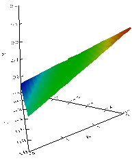
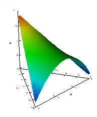
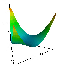
In Wilkinson's (2001) view, the multiple panel approach is less prone to erroneous perception than the multiple symbol approach. Wilkinson uses the comparison between bar charts in multiple panels and bar charts using multiple symbols in fewer panels as an example. He argues that in the latter, although the collapsing of dimensions into fewer panels could save space, it introduces a symbol choice problem. It is difficult to find symbols that are easily distinguishable for more than a few categories. On the other hand, bar charts in separate panels, which are more similar to Trellis displays, convey a higher degree of clarity. One drawback to the Trellis display is that the relationships depicted in each panel are bivariate. It does not give a wholistic sense of the multivariate relationship. We are not directly viewing the four-variable relationship in any one panel. This type of display requires viewing the combination of the bivariate plots to give the researcher a multivariate perspective. 2.3. 3D triangular plot The three-dimensional triangular plot, which is available in SyStat (SyStat Software, 2002), is used as an example of a spatial-oriented/model-driven visualization tool. Unlike the Trellis plot, raw data points are hidden and only the function is shown in the 3D triangular plot (Figure 5). It is important to note that the axes in this type of plot are collapsed using triangular coordinates. In the graph, there are four dimensions--three variables are depicted in the triangular coordinates on the "floor" of the data space, while the Y variable is represented as a vertical axis as in the Cartesian (rectangular) coordinate system. Since this type of data space combines features of both triangular and Cartesian coordinate systems, it is also named 3D triangular/rectangular coordinate system (Wilkinson, 1999). Triangular coordinates are also known as Barycentric coordinates, trilinear coordinates, and homogeneous coordinates. The technique was introduced by August Ferdinand Mobius in 1827 as a way to represent a point in the plane with respect to a given triangle. Although this new coordinate system was not appreciated at first, there are many interesting and useful applications (Dana-Picard, 2000; Diamond, 2001). Usually there are some constraints on the values of the three variables. Each variable can have a relative concentration between 0% and 100%. If A is at 100%, B and C must both be at 0%, and the point (100%, 0%, 0%) falls at one apex of the triangle. The three axes of three variables in the SyStat's density plot do not range from zero to one. A conversion takes place in the program that allows the variables to be represented simultaneously in the same data space. This results in a data space that includes a limited range of values across the predictor variables. Depending on the complexity of the variable relationship, this restricted area of the data space can be a major drawback of using this coordinate system. As in some other higher-dimensional graphs, in the density plot using Barycentric coordinates, the presence or absence of interaction effects can be judged by seeing whether the mesh surface is flat or curved. In Figure 5, it is apparent that there is no interaction. Meanwhile, Figure 6 is the depiction of a 2-way interaction, while Figure 7 shows a 3-way interaction.
The 3D triangular plot possesses a unique feature that is not present in other visualization tools presented here. A 3D triangular plot can display all four dimensions at the same time in one view. In a Trellis display, the user must swap the variables across each axis panel to get a thorough view of the data. In Maple 3D animation and SAS/Insight, which will be introduced in the next section, the fourth dimension is hidden unless the user requests it. Nonetheless, this high degree of condensation of dimensions comes at the expense of clarity. Although this type of graph can clearly distinguish no interaction, and 3-way interactions, it may be problematic to illustrate 2-way interactions. To be specific, even if there exists only an A*B interaction, the graph also gives an illusion of an A*C interaction because the slope of B against Y and the slope of C against Y seem to be affected by A.
3. Temporal-oriented Temporal-oriented visualization is also called Kinematic displays (Tukey & Tukey, 1988). As the name implies, temporal-oriented visualization techniques utilize variations across time to depict higher dimensions. In other words, not all variables are shown within the given space and time. The user must play an animation module to unveil more information (Wainer & Velleman, 2001). The "time" dimension can be designated as a variable where the values of the variable are used to illustrate change. 3.1. Animated graph in SAS/Insight SAS/Insight's animated graph (SAS Institute, 2001) is
one example of a temporal-oriented/data-driven plot. In
SAS/Insight, the fourth dimension is introduced as a
"time variable" (Figure 8). That is, the data points
representing a three-variable relationship suspended in a
three-dimensional space rendered on a computer screen are
each highlighted as the values of a fourth variable are
added sequentially from its lowest to highest value.
Figures 9a-9c depict the same dataset as you have seen in
Figure 4, in which a 3-way interaction is embedded. To
assist in the visualization process, SAS/Insight provides
several different visual fitting methods allowing the
researcher to examine the consistency between the data
and a model, namely, a parametric surface of the
researcher's choice (Figure 9a), a kernel density
smoothing surface (Figure 9b), and a spline smoothing
surface (Figure 9c). When the data are presented with a
parametric surface, it may not be easy to detect an
interaction effect. Nevertheless, in 9b and 9c,
there are slide bars for the user
to change the bandwidth in order to adjust the level of
smoothing, which indicates the change of the function as
a result of the interaction. After the 3D plot is drawn,
animation of the data points on the graph according to
the value change of another variable gives the point
cloud the appearance of points dancing about on the
graph, allowing the researcher to detect patterns and
structure in the multivariate relationship (Cheung,
2001).
However, this approach has at least three limitations. First, in order to make the pattern amongst data points emerge, a large data set is desirable because patterns are clearer when the observations dance in clusters across a dense cloud of points. A small data set may show a scattering dance among sparse points, and thus may fail to reveal any pattern at all. At first glance, this notion seems contradictory with some experimental findings. For example, Kareev, Lieberman and Lev (1997) found that the use of small samples led to more accurate detection of correlation. However, this is true if only a pairwise relationship is displayed. Yu (1994) also found empirically that the efficacy of visualization tools is a function of both the sample size and the number of dimensions. A large amount of data necessitates feature-rich visualization tools, and multiple dimensions require more observations. Second, the function overlay has been generated according to the first three variables in the plot. Therefore, the addition of the fourth variable does not alter the existing function. Although the points are highlighted, creating an illusion of movement, the surface remains static. A third, related limitation of the animated point cloud is that the addition of the animation variable to a 3-dimensional plot is not the same as viewing a four-variable relationship. The dancing effect of the animation has a different perceptual impact than that of the visual impression created from the pre-existing three-dimensional relationship. Further, it is the static visual associations that most people are accustomed to viewing and interpreting. Hence, the variable chosen as the animation variable may have unrevealed relationships with other variables involved. 3.2. Animated 3D plot in Maple Maple offers an animated 3D plot procedure (Waterloo Maple, 2001), which is one example of a temporal-oriented/model-driven visualization tool. Like SAS/Insight, in Maple the fourth variable is cast into a "time" variable. After a 3D mesh surface plot is generated, the mesh surface can be animated according to the varying values of the fourth variable. But unlike SAS/Insight, the surface is re-fitted based upon the fourth dimension, and there are no data points shown in the graph. Actually, Maple is capable of superimposing data points on a smoothed function, resulting in a plot very similar to the SAS/Insight plot prior to its animation of points 1. However, the data points are fixed to the original three dimensions in the Maple plot. The observations are not animated or highlighted according to the fourth variable, and it is only the mathematical function that has been input with defined variable ranges (not specified values) that determines the motion of the surface, which represents the four-variable relationship. Therefore, Maple's animated 3D plot is classified under the temporal-oriented/model-driven category of higher-dimension plots. In a typical 3D plot, the shape of the mesh surface determines the absence or presence of an interaction effect. A flat plane indicates the absence of an interaction effect while a warped surface is a sign of an interaction. In an animated 3D plot, even if the mesh surface is flat, one of the variables may still interact with the fourth variable when the slope changes according to the increment or decrement of the data value of the fourth variable (Figure 10).
When the mesh surface is curved, it is evident that there is a 2-way interaction. However, if the animated graph shows a moving mesh surface conditioning upon the fourth dimension, no doubt there is a 3-way interaction (Figure 11).
Other researchers using the geometric features of these displays include Cleveland and McGill (1984), who argue that Trellis displays are better than surface plots in terms of interpretation error rates. After they conducted a series of experiments on the efficacy of different graphical features, it was found that dots positioned along a common scale are the most salient features, while volume and color are more difficult to use as judgment factors. In this view, it may be predicted that Trellis displays are superior to function-driven plots because they use dots and each panel shares a common scale. Also, Wilkinson (1999) argues that although surface plots elicit a wholistic impression of a function, they are less useful for decoding individual values. On another occasion discussing surface plots, Wilkinson (1994) also points out that researchers can usually gain more information by displaying raw multivariate data directly, rather than by smoothing the trends in the swarm of observations. While we agree with Wilkinson's assessment to surface plots, Cleveland and McGill's assertion may be disputable.
4. Discussion In the following section, recommendations for appropriate use of various types of visualization tools will be given based upon our teaching, research, and consulting experience. 4.1 Nature of task and visualization tools The appropriateness of use of visualization tools is strongly tied to the nature of the task (Yu, 1994). A function-driven plot is practically useless to the researcher (exploratory or not) who hopes to find meaningful patterns in the data. Plotting the function superimposed over the data points can clearly be beneficial to many people, but a geometrical picture of the mathematical function alone does the researcher very little in the early stages of the regression analysis. Data-driven plots that show the observed relationship among the researchers' variables seem to be more appropriate when the objective is to explore and probe the data. A function plot becomes useful when the purpose is to display a complex relationship in a simple manner. For example, when one is teaching about the concept of interactions in regression, a common way to graphically illustrate the interaction is through plots of simple slopes (somewhat similar to a crude Trellis display) along with an ANOVA relationship demonstration. However, this requires some cognitive resourcefulness for most novice learners as the simple slope plots depict relationships that appear bivariate but are actually multivariate. In this case, a functional has the benefit of clarity in illustration. In the following we examine the merits and shortcomings of various graphs by the categories of teaching and research purposes. 4.2 Comparing Maple's 3D animation plot and SyStat's triangular plot for teaching purposes For teaching and presentation purposes, the temporal-based displays, such as the 3D animation plot in Maple, seem to have advantages over the currently available spatial-based graphs, such as the 3D triangular coordinate plot in SyStat. Most users are more familiar with the Cartesian space than the Barycentric space, and thus comprehension of the latter requires much more mental processing (and figure manipulation controls, which seems limited and cumbersome in the SyStat example). Although the 3D triangular plot allows the user to examine the plot from different perspectives with a rotation tool, no other tools are available. In this case, not only accessibility of manipulation tools is an issue, but also it seems that initial incomprehension discourages users from further exploration. The Maple 3D animation plot, conversely, seems to take linked displays to another level. The smooth motion of the animation makes the Maple graph appealing to most users. In addition, the degree of the user exploration is strongly tied to the accessibility of the features. In the Maple graph, all manipulation tools are available by a right-mouse click and all movie control buttons are visible in the top bar. Users tend to fully use the animation features during the exploration process. Further, it illustrates complex relationships among the many variables in a highly perceptible, wholistic manner. On the other hand, users who attempt to comprehend the graphs by rotating the plots into multiple 2D perspectives can be easily misled by the triangular plot. While in Maple's 3D animation plot the information conveyed by the multiple 2D perspectives could easily be converted, users fail to do so in the triangular plot. Also, the high degree of accessibility of manipulation tools in Maple allows more active exploration. For these reasons, it appears that the Maple 3D animation plot is more helpful in illustrating concepts such as regression interactions to learners, and for presenting complex relationships than the SyStat 3D triangular plot. 4.3 Comparing Splus's Trellis plot and SAS's animated plot for research purposes For research purposes, the spatial-based graphs, such as Trellis displays in S-Plus, are preferable over the temporal-based displays, such as the 3D animated plot in SAS/Insight. The multiple-view strategy employed by Trellis displays allows users to "divide and conquer" the problem by swapping the predictor and conditioning variables, allowing for the identification of complex relationships. Multiple dimensions are displayed, yet the static graph allows users to examine the conditioning panels one by one, and without any single variable being at a disadvantage. The user is also able to keep track of the changing values of the conditioning variables. However, usage of visualization tools requires an exploratory spirit. Many Trellis users tend to stay with the default view rather than swapping positions of predictors. As mentioned before, sometimes a relationship may be undetected in one view but could be revealed in another view. Moreover, some users tend to focus on the function (simple slope), but overlook the fit and residuals between the slope and the data points. To be fair, these problems are not inherent in the Trellis Plot; rather it is a matter of how to encourage users to conduct visualization in an exploratory fashion. In SAS/Insight, the "dance" of data points representing the four-variable relationship can be difficult to follow, especially since the values of the conditioning variables are located in a separate panel. Since highlighting the points across the values of the animation variable represent the association of the fourth variable with the pre-existing three-way relationship, the fourth variable requires a different perceptual operation than that which is used to interpret the initial three-way relationship. In other words, the variable chosen to represent the fourth dimension is not viewed in an equivalent, simultaneous manner with the first three variables in the data space. Evidently, this is cognitively demanding for users since it seems to require the viewers to simultaneously apply two distinct first-order factors of visual perception, a general visualization ability and spatial relations ability (see Carroll, 1993, for summaries of factor analytic studies in human perception). Additionally, given a continuous animation variable that includes numerous values each highlighted individually, the viewers likely exceed the short-term memory capacity prior to the completion of the animation effect and before any pattern recognition is possible. One must follow the pattern and the change in values simultaneously. As a result, the eyes necessarily miss a split second of the animation effect. Moreover, the existing relationship and the dancing of points that occur in that relationship could appear vastly different depending on the variables chosen for the initial three-variable plot. As a result, users' interpretation accuracy on the animated 3D plots in SAS/Insight is affected.
References Becker, R. A., Cleveland, W. S., & Shyu, M. J. (1996).The visual design and control of Trellis Display. Journal of Computational and Statistical Graphics, 5, 123-155. Bellman, R. E. (1961). Adaptive control processes. Princeton. NJ: Princeton University Press. Carroll, J. (1993). Human cognitive abilities: A survey of factor-analytical studies. New York: Cambridge Univeristy Press. Cheung, M. W. (2001 April). How to visualize the dance of the money bees using animated graphs in SAS/Insight. Paper presented at the Annual Meeting of SAS User Group International, Long Beach, CA. Chernoff, H. (1973). The use of faces to represent points in k-dimensional space graphically. Journal of the American Statistical Association, 68, 361-368. Clark, L. A., Cleveland, W. S., Denby, L., & Liu, C (1999). Competitive profiling displays: Multivariate graphs for customer satisfaction survey data. Marketing Research, 11, 25-33. Cleveland, W. S., & McGill, R. (1984). Graphical perception: Theory, experimentation, and application to the development of graphical methods. Journal of the American Statistical Association, 79, 531-554. Dana-Picard, T. (2000). Some applications of Barycentric computations. International Journal of Mathematical Education in Science & Technology, 31, 293-309. Diamond, W. (2001). Practical experiment designs for engineers and scientists. New York: Wiley. du Toit, S. H. C., Steyn, A. G. W. & Stumpf, R. H. (1986). Graphical exploratory data analysis. New York: Springer-Verlag. Fox, J. (1997). Applied regression analysis, linear models, and related methods. Thousand Oaks, CA: Sage. Insigthful, Inc. (2002). Splus Version 6. [Computer Software]. [On-line] Available URL: http://www.splus.com Mihalisin, T., Timlin, J., & Schegeler, J. (1991). Visualizing multivariate functions, data, and distributions. IEEE Computer Graphics and Applications, 11(3), 28-35. Jacoby, W. G. (1991). Data theory and dimensional analysis. Newbury Park, CA: Sage Publications. Jacoby, W. G. (1998). Statistical graphs for visualizing multivariate data. Thousand Oaks: Sage Publications. Kareev, Y., Lieberman, I., & Lev, M. (1997). Through a narrow window: Sample size and the perception of correction. Journal of Experimental Psychology, 126, 278-287. Mihalisim, T, Timlin, J. & Schedeler, J. (1991). Visualizing multivariate functions, data, and distributions. IEEE Computer Graphics and Applications, 11, 28-35. SAS Institute (2001). SAS/Insight Version 8.2. [Computer software] [On-line] Available URL: http://www.sas.com SyStat Software, Inc. (2002). SyStat Version 10. [Computer software] [On-line] Available URL: http://www.systat.com Tukey, P., & Tukey, J. (1988). Graphic display of data sets in 3 or more dimensions. In W. S. Cleveland (Ed.). The collected works of John Tukey: Volume V (pp. 189-288). Pacific Grove, CA: Wadsworth & Brooks. Wainer, J., & Velleman, P. (2001). Statistical graphs: Mapping the pathways of science. Annual Review of Psychology, 52, 305-335. Waterloo Maple. (2001). Maple Version 6. [Computer software]. [On-line] Available URL: http://www.maplesoft.com/ Wilkinson, L. (1993). Comments on W. S. Cleveland, a model for studying display methods of statistical graphs. Journal of Computational and Graphical Statistics, 2, 355-360. Wilkinson, L. (1994). Less is more: Two- and three-dimensional graphs for data display. Behavior Research Methods, Instruments, & Computers, 26, 172-176. Wilkinson, L. (1999). The grammar of graphics. New York: Springer. Wilkinson, L. (2001). Presentation Graphics. In N. J. Smelser, & P. B. Baltes (Eds.). International Encyclopedia of the Social and Behavioral Sciences, Volume 9 (pp. 6369-6379). New York : Elsevier. Yu, C. H. (1994). The interaction of research goal, data type, and graphical format in multivariate visualization. Unpublished dissertation, Tempe, AZ: Arizona State University. Yu, C. H. (1999). An Input-process-output structural framework for evaluating Web-based instruction. [On-line] Available URL: http://seamonkey.ed.asu.edu/~alex/teaching/assessment/structural.html Yu, C. H., & Behrens, J. T. (1995). Applications of scientific multivariate visualization to behavioral sciences. Behavior Research Methods, Instruments, and Computers, 2, 264-271.
Code used to create Maple 3D animation plots
Procedure for creating SyStat triangular plots (SyStat version 10):
Procedure for creating 3D plots in SAS/Insight:
Procedure for creating S-Plus Trellis displays:
Contact Information
| ||||||||||||||||||||||||||||||||||||
| Descriptors: Exploratory data analysis; data visualization; perception; user interface | ||||||||||||||||||||||||||||||||||||