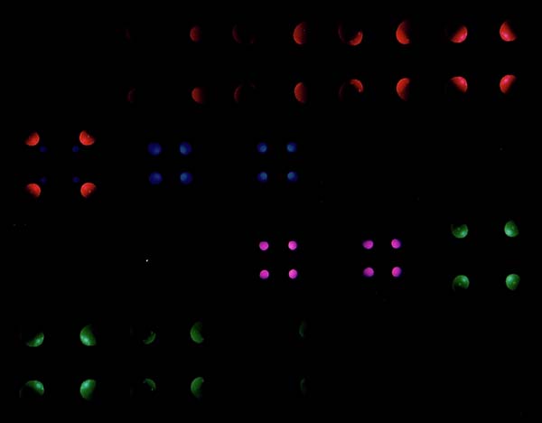
Figure 5.1
A 2x2x2 4D Raytrace Grid
Wireframe rendering has several advantages over other rendering methods, including simplicity of representation, speed of display, and ease of implementation. However, it cannot render solid objects, or objects that obscure one another. In addition, it cannot model other aspects of light propagation, such as shadows and reflections, which aid the user in understanding a given scene.
Other rendering techniques exist that solve the hidden surface problem and shadows by representing the objects with a tessellated mesh of polygons. These algorithms map the polygons to the viewport in a particular order to solve for hidden surfaces. These algorithms must also handle the cases of partially obscured polygons. However, these techniques are not easily extended to four-dimensional rendering. Instead of dealing only with planar polygons, the four-dimensional counterpart would have to deal with tessellating solids; thus, it would also have to properly handle intersecting solids with hidden volumes and solids that partially obscure one another. This is at best a difficult task in three-space; the four-space extension would be even more complex.
For these reasons, the raytracing algorithm was chosen to ``realistically'' render four-space scenes. Raytracing solves several rendering problems in a straight-forward manner, including hidden surfaces, shadows, reflection, and refraction. In addition, raytracing is not restricted to rendering polygonal meshes; it can handle any object that can be interrogated to find the intersection point of a given ray with the surface of the object. This property is especially nice for rendering four-dimensional objects, since many N-dimensional objects can be easily described with implicit equations.
Other benefits of raytracing extend quite easily to 4D. As in the 3D case, 4D raytracing handles simple shadows merely by checking to see which objects obscure each light source. Reflections and refractions are also easily generalized, particularly since the algorithms used to determine refracted and reflected rays use equivalent vector arithmetic.
The main loop in the raytracing algorithm shoots rays from the viewpoint through a grid into the scene space. The grid is constructed so that each grid element represents a voxel of the resulting image (see figure 5.1 for an illustration of a 2x2x2 ray grid). As a ray is ``fired'' from the viewpoint through the grid, it gathers light information by back-propagation. In this way raytracing approximates the light rays that scatter throughout the scene and enter the eye by tracing the rays back from the viewpoint to the light sources.
The recursive nature of raytracing, coupled with the fact that every voxel is sampled, makes raytracing very time consuming. Fortunately, extending the raytracing algorithm to four dimensions does not necessarily incur an exponential increase in rendering time. However, finding some ray-object intersections does entail a significant increase in computation. For example, determining the intersection of a four-space ray with a four-space tetrahedron is much more expensive than computing the intersection of a three-space ray with a three-space triangle. This increase of complexity does not necessarily occur with all higher-order object intersections, though. The hypersphere, for example, can be intersected with essentially the same algorithm as for the three-sphere (although vector and point operations must handle an extra coordinate).
The ray grid must be constructed so that each point on the grid corresponds to each pixel for 3D raytracing or voxel (volume element) for 4D raytracing. In four-dimensional raytracing, the grid is a three-dimensional parallelepiped spanned by three orthogonal vectors. Note that although in figure 5.1 it seems that a scene ray would pass through other voxels as it intersects each voxel center, scene rays do not lie in the same three-space (or hyperplane) as the ray grid. As a result, each scene ray intersects the ray grid only at the voxel centers.
The ray grid is constructed from the viewing parameters presented in section 3.2. These viewing parameters are the same as the viewing parameters used for the 4D wireframe viewer.
The viewpoint is the point of origin for the scene rays, so it must be outside of the ray grid. Since the to-point is the point of interest, it should be centered in the 4D ray grid.
Now that we have the center of the ray grid, we need to establish the basis vectors of this grid. Once we do that, we can index a particular voxel in the grid for the generation of scene rays.
The up-vector and over-vector are used to form two of the grid basis vectors (after proper scaling). Since the line of sight must be perpendicular to the ray grid, we can generate the third basis vector by forming the four-dimensional cross product of the line of sight with the up-vector and over-vector. Note that in four-space, a ray can pass through any point within the cube without intersecting any other point.
The grid basis vectors are computed as follows:
               From - To
         S = -------------
             ||From - To||

               cross4 (Over, Up, S)
        Bz = ------------------------
             ||cross4 (Over, Up, S)||

               cross4 (Bz, S, Over)
        By = ------------------------
             ||cross4 (Bz, S, Over)||

        Bx = cross4 (By, Bz, S)
At this point, S is the unit line-of-sight vector, and Bx, By & Bz are
the unit basis vectors for the ray grid. What we need to do now is to to scale
these vectors. There are two additional sets of parameters that govern the
construction of the ray grid. These are the the number of voxels along each axis
of the grid (the resolution of the ray grid), and the shape of each voxel (the
aspect ratios). In addition, we need to incorporate the viewing angle.
The resolution of the grid cube is given by the parameters Rx, Ry and Rz, which specify the number of voxels along the width, height and depth of the cube, respectively. The aspect ratio of each voxel is given by the parameters Ax, Ay and Az. These parameters specify the width, height and depth of each voxel in arbitrary units (these numbers are used only in the ratio). For example, an aspect ratio of 1:4:9 specifies a voxel that is four times as high as it is wide, and that is 4/9ths as high as it is deep.
The ray grid is centered at the to-point; we use the viewing angle to determine the ray-grid size. As mentioned earlier, the viewing angle corresponds to the X axis. The other axes are sized according to the resolution and aspect ratios. Determining the proper scale of the grid X axis is easily done from the viewing angle
Lx = 2 ||From-To|| tan(theta4/2)where theta4 is the 4D viewing angle, and Lx is the width of the ray grid. The other dimensions of the ray grid are determined by Lx, the aspect ratios, and the resolutions:
                Ry Ay                    Rz Az
        Ly = Lx -- --,    and    Lz = Lx -- --
                Rx Ax                    Rx Ax
Thus, Lx, Ly and Lz are the lengths of each edge of the ray grid, and the
grid basis vectors are scaled with these lengths to yield Gx = Lx Bx, Gy = Ly By, and Gz = Lz Bz.The main ray loop will start at a corner of the ray grid and scan in X, Y and Z order, respectively. The origin of the grid (each basis vector zero) is given by
                 Gx + Gy + Gz
        O = To - ------------.
                      2
The incremental grid vectors are used to move from one grid voxel to
another. They are computed by dividing the grid-length vectors by the respective
resolution: Gx Gy Gz
Dx = --, Dy = --, Dz = --.
Rx Ry Rz
Finally, the grid origin is offset by half a voxel, in order that the
voxel centers are sampled. Dx + Dy + Dz
O = O + ------------
2
The main raytracing procedure looks like this: Vector4 Dx,Dy,Dz; // Grid-Traversal Vectors
Point4 From4; // 4D Viewpoint
Point4 Origin; // Grid Origin Corner
int Rx,Ry,Rz; // Grid Resolutions
void FireRays (void)
{
int i,j,k; // Grid Traversal Indices
Vector4 T; // Scratch Vector
Ray4 ray; // 4D View Ray
for (i=0; i < Rx; ++i) {
for (j=0; j < Ry; ++j) {
for (k=0; k < Rz; ++k) {
T = Origin + i*Dx + j*Dy + k*Dz;
VecCopy (ray.origin, From);
VecSub (ray.direction, T,ray.origin);
// Recursively fire sample rays into the scene.
Raytrace (ray);
}
}
}
}
Each ray is propagated throughout the scene in the following manner:
The reflection and refraction rays mentioned in the previous section are generated in the same way as they are for 3D raytracing, with the exception that the vector arithmetic is of four dimensions rather than three. Since reflection and refraction rays are confined to the plane containing the normal vector and the view vector, reflection and refraction rays are given by the following equations for raytracing in any dimension higher than one.
Refer to figure 5.2 for a diagram of the reflection ray.
The equation of the reflection ray is given by is
R = D - 2 (N·D) Nwhere R is the resulting reflection ray, D is the unit direction of the light ray towards the surface, and N is the unit vector normal to the surface. Refer to [Foley 87] for a derivation of the reflection equation.
The refraction ray T is given by
        T = dC + (1-d)(-N)

               D
        C = -------
            ||N·D||

                              1
        d = ------------------------------------
            sqrt(((r1/r2)² * ||C||²) - ||C+N||²)
where T is the refraction ray, D is the unit direction of the light ray towards the surface, N is the unit normal vector to the surface, r1 is the index of refraction of the medium containing the light ray, and r2 is the index of refraction of the object. Note that this equation does not yield a unit vector for T; T must be normalized after this equation. Refer to [Hill 90] for a derivation of this formula.
The illumination equations for four-dimensional raytracing are the same as those for raytracing in three dimensions, although the underlying geometry is changed. A simple extended illumination equation is as follows:
                    N
                    __
                    \                           n
        I = Ia Ka + /  IL(Kd cos(theta) + Ks cos (alpha)) + Ks Ir + Kt It.
                    ~~
                    L=1
The values used in this equation are
| Ia [RGB] | Global ambient light. |
| IL [RGB] | Light contributed by light L. |
| Ir [RGB] | Light contributed by reflection. |
| It [RGB] | Light contributed by transmission (refraction). |
| Ka [RGB] | Object ambient color. |
| Kd [RGB] | Object diffuse color. |
| Ks [RGB] | Object reflection color. |
| Kt [RGB] | Object transparent color. |
| n [Real] | Phong specular factor. |
| N [Integer] | Number of light sources. |
Refer to figure 5.3 for a diagram of the illumination vectors and components. The angle theta between the surface normal vector and the light direction vector determines the amount of diffuse illumination at the surface point. The angle alpha is the angle between the reflected light vector and the viewing vector, and determines the the amount of specular illumination at the surface point. These angles are given by the following formulas.
        cos(theta) = N·L(lambda)

        cos(alpha) = R·L(lambda)
If cos(theta) is negative, then there is no diffuse or specular illumination at the surface point. If cos(theta) is non-negative and cos(alpha) is negative, then the surface point has diffuse illumination but no specular illumination.
In the summation loop, a ray is fired from the surface point to each light source in the scene. If this shadow ray intersects any other object before the light source, then the contribution from that light source is zero; I(lambda) for light source lambda is set to zero. If no object blocks the light source, then I(lambda) is used according to the type of light source.
The raytracer developed for this research implements both point and directional light sources. For directional light sources, the vector L(lambda) is constant for all points in the scene. For point light sources, L(lambda) is calculated by subtracting the point light source location from the surface point. Both of these light sources are assigned a color value (I(lambda)).
The fundamental objects implemented in the 4D raytracer include hyperspheres, tetrahedra and parallelepipeds. The intersection algorithms for each of these objects takes a pointer to the object to be tested plus the origin and unit direction of the ray. If the ray does not intersect the object, the function returns false. If the ray hits the object, the function returns the intersection point and the surface normal at the intersection point.
Some objects, such as hyperspheres, can have zero, one or two intersection points. More complex objects may well have many more intersection points. The intersection functions must return the intersection point closest to the ray origin (since other intersection points would be obscured by the nearest one.)
The hypersphere is one of the simplest four-dimensional objects, just as the three-sphere is among the simplest objects in 3D raytracers. Like the three-sphere, the four-sphere is specified by a center point and a radius.
The implicit equation of the four-sphere is
(Sx - Cx)² + (Sy - Cy)² + (Sz - Cz)² + (Sw - Cw)² - r² = 0
where r is the radius of the four-sphere, C is the center of the sphere, and S is a point on the surface of the sphere.
Obtaining the normal vector from the intersection point is a trivial matter, since the surface normal of a sphere always passes through the center. Hence, for an intersection point I, the surface normal at I is given by N = I - C.
Calculating the intersection of a ray with the sphere is also fairly straight-forward. Given a ray defined by the equation r = P + tD, where P is the ray origin, D is the unit ray direction vector, and t is a parametric variable, we can find the intersection of the ray with a given hypersphere in the following manner:
        (Cx - Sx)² + (Cy - Sy)² + (Cz - Sz)² +  (Cw - Sw)² - r² = 0

        ||C - S||² - r² = 0
Substitute the ray equation into the surface value to get
        ||C - (P + tD)||² - r² = 0

        ||(C - P) - tD||² - r² = 0

        ||V - tD||² - r² = 0         where V = C - P

        (Vx - tDx)² + (Vy - tDy)² + (Vz - tDz)² + (Vw - tDw)² - r² = 0

        t²(Dx² + Dy² + Dz² + Dw²) - 2t (VxDx + VyDy + VzDz + VwDw)

            + (Vx² + Vy² + Vz² + Vw²) - r² = 0
This simplifies to
t²(D·D) - 2t (V·D) + (V·V - r²) = 0.
Since D is a unit vector, this equation further simplifies to
t² - 2t (V·D) + (V·V - r²) = 0.
The quadratic formula x² - 2bx + c = 0 has roots b ± sqrt(b² - c). So, solving for t, we get
t = (V·D) ± sqrt((V·D)² - (V·V - r²)).
The intersection point is given by plugging the smallest non-negative solution for t into the ray equation. If there is no solution to this equation (e.g., the quantity under the square root is negative), then the ray does not intersect the hypersphere.
The pseudo-code for the ray-hypersphere intersection algorithm follows.
    function  HitSphere: Boolean  (
	ray:       Ray4,
	sphere:    Sphere4,
	intersect: Point4,
	normal:    Vector4
    )
	bb:    Real    Quadratic Equation Value
	V:     Vector4 Vector from Ray Origin to Sphere Center
	rad:   Real    Radical Value
	t1,t2: Real    Ray Parameter Values for Intersection

	V <- sphere.center - ray.origin
	bb <- Dot4(V,ray.direction)
	rad <- (bb * bb) - Dot4(V,V) + sphere.radius_squared

	If the radical is negative, then no intersection.

	if rad < 0
	    return false

	rad <- SquareRoot(rad)
	t2  <- bb - rad
	t1  <- bb + rad

	Ensure that t1 is the smallest non-negative value (nearest point).

	if t1 < 0 or (t2 > 0 and t2 < t1)
	    t1 <- t2

	If sphere is behind the ray, then no intersection.

	if t1 < 0
	    return false

	intersect <- ray.origin + (t1 * ray.direction)
	normal  <- (intersect - sphere.center) / sphere.radius

	return true

    endfunc HitSphere
The tetrahedron is to the 4D raytracer what the triangle is to the 3D raytracer. Just as all 3D objects can be approximated by an appropriate mesh of tessellating triangles, 4D objects can be approximated with an appropriate mesh of tetrahedra. Of course, the tessellation of 4D objects is more difficult (e.g. how do you tessellate a hypersphere?), but it does allow for the approximation of a wide variety of objects.
In the fourth dimension, the tetrahedron is ``flat'', i.e. it has a constant normal vector across its volume. Any vector embedded in the tetrahedron is perpendicular to the tetrahedron normal vector.
The tetrahedron is specified by four completely-connected vertices in four-space. A tetrahedron in which the four vertices are coplanar is a degenerate tetrahedron; it is analogous to a triangle in three-space with colinear vertices. The 4D raytracer should ignore degenerate tetrahedra as invisibly thin.
Since the tetrahedron normal is constant, pre-compute this vector and store it in the tetrahedron description before raytracing the scene. The normal is computed by finding three independent vectors on the tetrahedron and crossing them to compute the orthogonal normal vector.
        B1 = V1 - V0,

        B2 = V2 - V0,

        B3 = V3 - V0, and

              X4(B1,B2,B3)
        N = ----------------
            ||X4(B1,B2,B3)||
where V0, V1, V2, and V3 are the tetrahedron vertices and N is the unit normal vector.
Finding the intersection point of a ray and tetrahedron is much more difficult than for the hypersphere case. This is primarily because it requires the solution of a system of three equations and three unknowns to find the barycentric coordinates of the intersection point.
Once the barycentric coordinates of the intersection point are known, they can be used to determine if the point lies inside the tetrahedron, and also to interpolate vertex color or vertex normal vectors across the hyperface of the tetrahedron (Gouraud or Phong shading, respectively). For further reference on barycentric coordinates, refer to [Farin 88] and [Barnhill 84] (particularly the section on simplices and barycentric coordinates).
The method used to find the barycentric coordinates of the ray-hyperplane intersection with respect to the tetrahedron is an extension of the algorithm for computing barycentric coordinates of the ray-plane intersection with respect to the triangle, presented in [Glassner 90].
Again, the ray is specified by the equation P + tD, where P is the ray origin, D is the unit direction vector, and t is the ray parameter. For each point Q on the tetrahedron, Q·N is constant. Let d = - V0·N. Thus, the hyperplane is defined by N·Q + d = 0, where the tetrahedron is embedded in this hyperplane.
First compute the ray-hyperplane intersection with t = - (d + N·P) / (N·D). If N·D is zero, then the ray is parallel to the embedding hyperplane; it does not intersect the tetrahedron. If t < 0, then the embedding hyperplane is behind the ray, so the ray does not intersect the tetrahedron.
Now compute the ray-hyperplane intersection with relation to the tetrahedron. The barycentric coordinates of the intersection point Q is given by the equation
        ____         _____        _____         _____
        V0 Q = alpha V0 V1 + beta V0 V2 + gamma V0 V3.      [5.5.2a]
The ray-hyperplane intersection point Q is inside the tetrahedron if
Equation 5.5.2a can be rewritten as
    [5.5.2b]

    +-      -+         +-       -+        +-       -+         +-       -+
    |Qx - V0x|         |V1x - V0x|        |V2x - V0x|         |V3x - V0x|
    |Qy - V0y| = alpha |V1y - V0y| + beta |V2y - V0y| + gamma |V3y - V0y|.
    |Qz - V0z|         |V1z - V0z|        |V2z - V0z|         |V3z - V0z|
    |Qw - V0w|         |V1w - V0w|        |V2w - V0w|         |V3w - V0w|
    +-      -+         +-       -+        +-       -+         +-       -+
To simplify the solution for these coordinates, we project the tetrahedron to one of the four primary hyperplanes (XYZ, XYW, XZW or YZW). To make this projection as ``large'' as possible (to ensure that we don't ``flatten'' the tetrahedron by projecting it to a perpendicular hyperplane), find the dominant axis of the normal vector and use the hyperplane perpendicular to the dominant axis. In other words the normal to the major hyperplane is formed by replacing the normal coordinate that has the largest absolute value with zero. For example, given a normal vector of <3, 1, 7, 5>, the dominant axis is the third coordinate, and the hyperplane perpendicular to <3, 1, 0, 5> will yield the largest projection of the tetrahedron. Once again, since the normal vector is constant, the three non-dominant coordinates (X, Y, and W for the above example) should be stored for future reference. Refer to the intersection algorithm for an illustration of this.
The hyperplane equation is then reduced to three coordinates, i, j, and k (X, Y & W for the previous example), so equation [5.5.2b] is reduced to
    [5.5.2c]

    +-      -+         +-       -+        +-       -+         +-       -+
    |Qi - V0i|         |V1i - V0i|        |V2i - V0i|         |V3i - V0i|
    |Qj - V0j| = alpha |V1j - V0j| + beta |V2j - V0j| + gamma |V3j - V0j|.
    |Qk - V0k|         |V1k - V0k|        |V2k - V0k|         |V3k - V0k|
    +-      -+         +-       -+        +-       -+         +-       -+
Now find alpha, beta, and gamma by solving the system of three equations and three unknowns; these are the barycentric coordinates of the intersection point Q relative to the tetrahedron. The fourth barycentric coordinate is given by (1 - alpha - beta - gamma).
In order for the tetrahedron to contain the ray-hyperplane intersection point, the following equations must be met:
        alpha >= 0,  beta >= 0,  gamma >= 0, and

        (alpha + beta + gamma) <= 1.
If any of the barycentric coordinates are less than zero, or if the barycentric coordinates sum to greater than one, then the ray does not intersect the tetrahedron.
Once alpha, beta and gamma are known for the point of intersection, the ray-hyperplane intersection point Q can be found by the following equation:
Q = (1 - alpha - beta - gamma)V0 + alpha V1 + beta V2 + gamma V3.
The following pseudo-code implements the ray-tetrahedron intersection algorithm.
    function  HitTet: Boolean (
	ray:       Ray4,
	tet:       Tetrahedron,
	intersect: Point4,
	normal:    Vector4
    )
	A11,A12,A13: Real    Equation System Matrix Values
	A21,A22,A23: Real
	A31,A32,A33: Real
	b1, b2, b3 : Real    Equation System Results
	rayt:        Real    Ray Parameter Value for Intersection
	x1, x2, x3 : Real    Equation System Solution

	Compute the intersection of the ray with the hyperplane containing
	the tetrahedron.

	rayt <- Dot4 (tet.normal,ray.direction)
	if rayt < 0 return false

	rayt <- - (tet.HPlaneConst + Dot4 (tet->normal,ray.origin)) / rayt
	if rayt < 0 return false

	Calculate the intersection point of the ray and embedding hyperplane.

	intersect <- ray.origin + (rayt * ray.direction)

	Calculate the equation result values.  Note that the dominant axes are
	precomputed and stored in tet.axis1, tet.axis2, and tet.axis3.

	b1  <- intersect[tet.axis1] - tet.V0[tet.axis1]
	b2  <- intersect[tet.axis2] - tet.V0[tet.axis2]
	b3  <- intersect[tet.axis3] - tet.V0[tet.axis3]

	Calculate the matrix of the system of equations.  Note that the
	vectors corresponding to V1-V0, V2-V0, and V3-V0 have been precomputed,
	and are stored in the fields tet.vec1, tet.vec2, and tet.vec3.

	A11 <- tet.vec1[tet.axis1]
	A12 <- tet.vec1[tet.axis2]
	A13 <- tet.vec1[tet.axis3]

	A21 <- tet.vec2[tet.axis1]
	A22 <- tet.vec2[tet.axis2]
	A23 <- tet.vec2[tet.axis3]

	A31 <- tet.vec3[tet.axis1]
	A32 <- tet.vec3[tet.axis2]
	A33 <- tet.vec3[tet.axis3]

	Solve the system of three equations and three unknowns.

	SolveSys3 (A11,A12,A13, A21,A22,A23,  A31,A32,A33, b1,b2,b3, x1,x2,x3)

	if x1 < 0 or x2 < 0 or x3 < 0 or (x1+x2+x3) > 1
	    return false

	Set the intersection barycentric coordinates.

	tet.bc1 <- x1
	tet.bc2 <- x2
	tet.bc3 <- x3

	normal <- tet.normal  The tetrahedron normal is precomputed.
	return true

    endfunc HitTet
The tetrahedron can be rendered with Flat, Gouraud or Phong shading, since the barycentric coordinates of the intersection points are known. For Gouraud shading with vertex colors C0, C1, C2 and C3 corresponding to V0, V1, V2 and V3, respectively, the color Cintersect of the intersection point is given by
Ci = (1 - alpha - beta - gamma)C0 + alpha C1 + beta C2 + gamma C3.
Phong shading can be used to interpolate the normals N0, N1, N2 and N3 to find the interpolated normal Ni of the intersection point with this equation:
Ni = (1 - alpha - beta - gamma)N0 + alpha N1 + beta N2 + gamma N3.
The parallelepiped was included in the 4D raytracer because of the similarities between the parallelepiped and the tetrahedron. Like the tetrahedron, the parallelepiped is specified with four vertices. The intersection algorithm for the parallelepiped differs from the algorithm for the tetrahedron in a single comparison; hence its inclusion in the set of fundamental objects is relatively free if the tetrahedron is already provided.
Like the tetrahedron, the normal vector for the parallelepiped is constant and is given by the 4D cross product of the three vectors
        _____   _____      _____
        V1 V0,  V2 V0, and V3 V0.
The intersection point is computed in the same manner as for the tetrahedron, with the exception that the barycentric coordinates alpha, beta and gamma must meet slightly different criteria:
        0 <= alpha <= 1,
        0 <= beta  <= 1, and
        0 <= gamma <= 1.
If the tetrahedron and parallelepiped data structures are defined properly, the intersection routine for the tetrahedron can also solve for ray-parallelepiped intersections. The only difference is that for the parallelepiped, the barycentric coordinates alpha, beta, and gamma can sum to greater than one, whereas the tetrahedron requires that their sum does not exceed one.
The output of the 4D raytracer is a 3D grid of voxels, where each voxel is assigned an RGB triple. This data can be thought of as set of scanplanes, or as a 3D scalar field of RGB data.
One way to display this data is to present it in slices, either individually, or as a tiled display of scanplanes. Producing an animation of the data a scanplane at a time is also a good method for displaying the image cube, although it would be best displayed this way under user interaction (e.g. by slicing the voxel field under mouse control).
[Drebin 88] also suggests a method of visualization that would be very appropriate for this sort of data, where the voxel field is presented as a field of colored transparent values. Although the algorithm as presented takes real-valued voxels, rather than RGB voxels, the RGB output data can be converted to greyscale (one common equation is Intensity = 0.299 Red + 0.587 Green + 0.114 Blue, as given in [Hall 89]). The resulting single-valued scalar field can then be visualized with a variety of algorithms, including also [Chen 85], [Kajiya 84], and [Sabella 88].
It's also possible to produce single scanplanes from the 4D raytracer, and use two of these as the left and right eye images for stereo display, although the presence of an extra degree of parallax makes this method less helpful than might initially be thought.
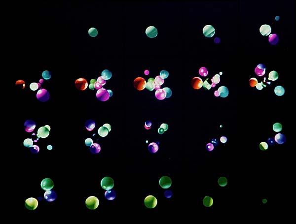
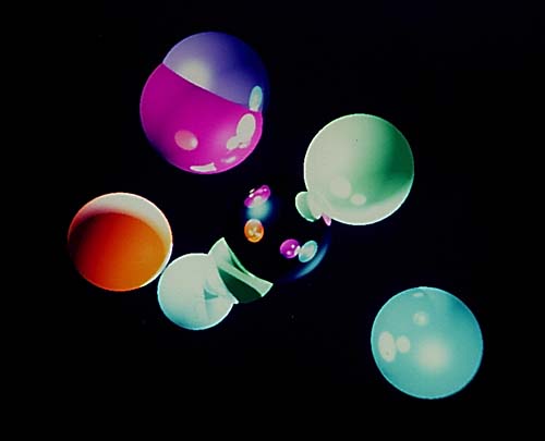
Several 4D raytraced images are included in this section. Figure 5.4 is the ray-traced image of a random distribution of four-spheres. All of the four-spheres have the same illumination properties; only the colors and positions are different. Notice that the Phong specular illumination manifests itself at different slices of the image cube.
One way to explain this phenomena is that just as the 3D to 2D projection of a shiny sphere yields a 2D phong spot embedded somewhere in the 2D projection of the sphere, a shiny four-sphere is projected to 3D with a 3D phong region embedded somewhere in the 3D projection of the four-sphere.
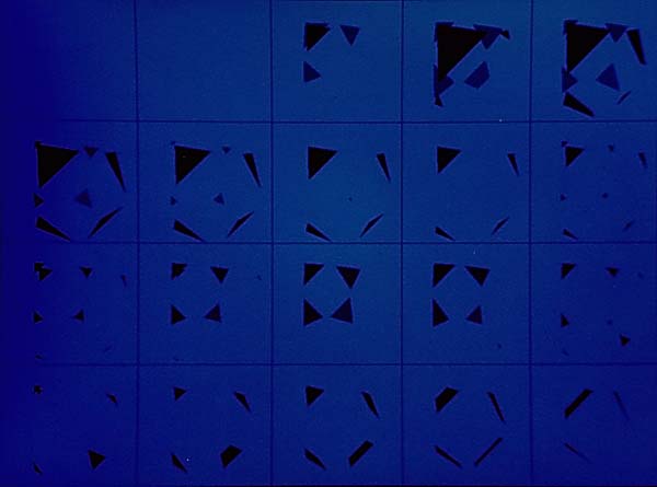
Figure 5.5 is the sliced image cube of sixteen four-spheres of radius 0.5 positioned at the vertices of a four-cube at locations <±1.25, ±1.25, ±1.25, ±1.25>.
Figure 5.6 is similar to figure 5.5, except that four-tetrahedrons are placed at the vertices rather than four-spheres. The four-tetrahedrons are oriented so that the normal of each four-tetrahedron is aimed at the center of the four-cube, and the four-tetrahedron vertices lie on the four-cube edges.
| Previous Chapter | Table of Contents | Next Chapter |