Figure 4.1
3D Eye Coordinates
Projection from four-space to a two-space region involves an additional projection compared to the usual display of three-dimensional wireframe data. Both the 3D projection and the additional 4D projection can be governed by independent sets of viewing parameters.
The first step of the 4D wireframe display process is to project the 4D vertices from four-space to an intermediate three-dimensional region. This projection uses the four dimensional viewing parameters discussed in section 3.2, and can be either a perspective projection or a parallel projection.
The next step is to take the projected vertices (now in three-space) and project them once more to the 2D viewport rectangle. This projection is determined by the three dimensional viewing parameters presented in section 3.1, and can also be either parallel or perspective. Once the vertices have been projected to screen coordinates, each edge of the wireframe is displayed.
There are several methods of projecting three-space points to a two-dimensional viewport. The method used and extended for this research is found in [Foley 87], and involves a vector subtraction and a multiplication between a 3-vector and a 3x3 matrix for each projected point.
The first step in projecting a 3D point is to convert its absolute ``world'' coordinates to viewer-relative ``eye'' coordinates. In the left-handed eye coordinate system, the eye-point is at the origin, the line-of-sight corresponds to the Z axis, the up-vector corresponds to the Y axis, and the X axis is orthogonal to the resulting Y and Z axes. Refer to figure 4.1 for a diagram of the eye-coordinate system.
To convert a 3D point to 3D eye coordinates, one must first establish the vector from the eye-coordinate origin to the point by subtracting the from-point from the 3D vertex. Then the vector difference is rotated so that the to-point lies on the Z axis of the eye-coordinate system, and the up-vector lies on the Y axis. This is accomplished by multiplying the vector difference by the transformation matrix. The 3x3 transformation matrix has column vectors A, B and C, where A, B and C correspond to the X, Y, and Z axes in eye coordinates, respectively. The equations for these vectors are
              To - From
        C = -------------,
            ||To - From||

              Up x C
        A = ----------, and
            ||Up x C||

        B = C x A,
where To is the to-point, From is the from-point, Up is the up-vector, and
the original world coordinates are supplied in the left-handed coordinate
system. For the right-handed coordinate system, the cross product order for
column vectors A and B would be reversed.
The procedure for computing the transformation matrix is given in the following algorithm. Note that Norm3(V) returns the vector norm of the 3-vector parameter V, and Cross3(U,V,W) assigns to U the 3-vector cross product of the parameter vectors V and W.
    // The parameters a, b and c are the resulting transformation matrix
    // column vectors.

    void Calc3Matrix (
        Point3   From,      // Looking From This Point
        Point3   To,        // Point of Interest
        Vector3  Up,        // Direction Up
        Vector3 *Va,        // Return Vector A
        Vector3 *Vb,        // Return Vector B
        Vector3 *Vc)        // Return Vector C
    {
        // Get the normalized Vc column-vector.

        VecSub (Vc, To, From);
        norm = Norm3 (Vc);
        if (norm == 0)
            Error ("To point and From point are the same.");
        VecScale (Vc, 1/norm);

        // Calculate the normalized Va column-vector.

        VecCross3 (Va, Vc, Up3);
        norm = Norm3 (Va);
        if (norm == 0)
            Error ("Up is parallel to the line of sight.");
        VecScale (Va, 1/norm);

        // Calculate the Vb column-vector.

        Cross3 (Vb, Va, Vc);
    }
Once the A, B and C vectors (corresponding to Va, Vb and Vc in the
pseudo-code above) are calculated, all 3D points can be transformed from 3D
world coordinates to 3D eye coordinates as follows: +- -+
| Ax Bx Cx |
P' = [(Px-Fx) (Py-Fy) (Pz-Fz)] | Ay By Cy |
| Az Bz Cz |
+- -+
where Fx, Fy and Fz are the X, Y and Z coordinates of the from-point, P is
the original data point in 3D world coordinates, and P' is the transformed data
point in eye coordinates.
We can now use the resulting 3D eye coordinates to project the 3D points to a two-dimensional rectangle. What we want is a projection that maps 3D points that lie in the 3D viewing frustum to the [-1,+1] x [-1,+1] rectangle. This rectangle will later be mapped to the viewport on the display device.
The projection from three-space to the 2D rectangle can be either a parallel projection or a perspective projection.
Parallel projection maps objects to the viewport in such a way that distant objects appear the same size as near objects. This is the effect that you'd get if the eye-point was infinitely far away from the object to be viewed. In the simple case where the projection plane is parallel to the XY plane, parallel projection can be achieved by dropping the Z coordinate (this is the case for eye coordinates). Scaling the projection to fit the [-1,+1] x [-1,+1] rectangle makes it easy to project the image to the viewport.
Perspective projection is the more natural of the two projections. With perspective projection, objects that are far away appear smaller than objects that are near. In the simple case, perspective projection is achieved by dividing by the Z coordinate. Perspective projection should map all data points that lie in the viewing frustum to the [-1,+1] x [-1,+1] rectangle.
When using parallel projection, the equation of the data point's normalized screen coordinates (from eye coordinates) is given by the following pair of equations:
             P'x                P'y        [4.2a]
        Tx = ---    and    Ty = ---,
             R3                 R3
where P' is the 3D point in eye coordinates, R3 is the radius of the set
of 3D points centered at the 3D to-point, and T is the 2D parallel projection of
P' to the [-1,+1] x [-1,+1] rectangle. Dividing by R3 ensures that the parallel
projection fills the viewport as much as possible without extending past the
viewport boundaries.
For the perspective projection of point P', consider figure 4.2.
To calculate the perspective projection of point P', we need to project the point to the viewplane and then to normalize the values so that points on the Z axis are projected to X (or Y) = 0, and so that the values of X (or Y) range from -1 to +1. The X axis value from figure 4.2 is calculated by noting that P'x/P'z = T'x/T'z. We can let T'z = 1 if the viewing angle is still preserved. Thus, T'x = P'x/P'z. To normalize T'x, note that the maximum possible value of T'x on the viewing plane occurs at T'x/T'z = tan(theta3/2), or T'x = tan(theta3/2). Thus, the equations for the normalized perspective projection T are given by
                P'x                               P'y           [4.2b]
    Tx = -----------------     and     Ty = -----------------
         P'z tan(theta3/2)                  P'z tan(theta3/2)
where theta3 is the 3D viewing angle and T is the normalized perspective
projection of P' to the [-1,+1] x [-1,+1] rectangle. Note that in the equations
presented in this chapter, the viewport is assumed to be square, so the viewing
angle for the horizontal plane and the viewing angle for the vertical plane are
the same. This assumption will also be held and extended for the 4D to 3D
projection covered later.
Now that we have the points in the [-1,+1] x [-1,+1] rectangle, we'll need to map them to the viewport on the display device. This viewport is specified by the parameters
                  Lx                         Ly          [4.2c]
        Sx = Cx + ---Tx,    and    Sy = Cy + ---Ty.
                   2                          2
Putting this all together, we get the following algorithm. Note that the
function Dot3(U,V) returns the dot product of the two 3-vector
parameters U and V. int NumVerts; // Number of 3D Vertices
double Radius; // Radius of Vertices About the To3 Point
Vector3 Va,Vb,Vc; // Viewing-Transformation Column Vectors
Radians Vangle; // 3D Viewing Angle
Vertex3 *VertList; // The Set of 3D Vertices
void ProjectToScreen (
float Cx, float Cy,
float Lx, float Ly,
ProjectionType proj_type)
{
double S, T; // Divisor Values
Vector3 V; // Scratch Vector
if (proj_type == PARALLEL)
S = 1 / Radius;
else
T = 1 / tan (Vangle / 2);
for (i=0; i < NumVerts; ++i) {
V = VertList[i].Position - From;
if (proj_type == PERSPECTIVE)
S = T / Dot3 (V, Vc);
VertList[i].Screen[x] = Cx + (Lx * S * Dot3 (V, Va));
VertList[i].Screen[y] = Cy + (Ly * S * Dot3 (V, Vb));
}
}
In this section, we extend the ideas and equations presented in section 4.2 to cover the projection of points from four-space to the intermediate 3D region.
It is possible to combine the 4D to 3D and 3D to 2D projections into a single step, but this approach lacks the flexibility of the following two-step approach. The two-step approach allows the user to independently specify viewing parameters for each projection, and to view the 3D projection from different angles while maintaining a constant 4D view.
Since the 4D to 2D projection takes place in two discrete steps, we'll need to specify an intermediate 3D region for the projection to 3D coordinates. For this research, the unit cube (edge length two) centered at the origin, with vertices <±1, ±1, ±1> was chosen as the intermediate region.
As in the 3D to 2D projections, the 4D data points can be projected to 3D space with either a perspective projection or a parallel projection. Neither of these projections are more ``intuitive'' than the other, but a perspective projection will yield smaller 3D line segments for edges that are farther from the 4D viewpoint. As an example of the differences between these projections, see section 4.6.
Changing the 3D projection type between perspective and parallel projection does not produce as dramatic (or puzzling) a change as for the 4D projection. However, switching back and forth can also provide a bit more understanding of the 4D-projected object.
The projection from 4D to 3D needs to be clipped at a minimum against the W=0 eye-coordinate plane. If both vertices have negative W eye-coordinate components, the edge should not be displayed. If both vertices have non-negative W components, then the edge can be displayed normally. If only one of the two vertices of a given edge has a negative W component, then the edge needs to be clipped to the W plane. This can be done by finding the intersection of the edge with the W plane and setting the vertex with the negative W component to the intersection point.
Since the 4D edges are projected to an arbitrary 3D region, it is not critical that they be clipped against the 4D viewing frustum. Edges that lie outside of the viewing frustum will lie outside the 3D region.
The first step of the 4D to 3D projection is to transform the vertices from their 4D world coordinates to the 4D eye coordinates. Refer to figure 4.3 for an illustration of the 4D eye coordinates.
As in the 3D to 2D projection, this transformation is accomplished with a transformation matrix. The 4D viewing transformation matrix is composed of the column vectors A, B, C and D, which correspond to the X, Y, Z and W eye-coordinate axes, respectively. The equations for these column vectors are
              To - From
        D = -------------,
            ||To - From||

              X4(Up,Over,D)
        A = -----------------,
            ||X4(Up,Over,D)||

              X4(Over,D,A)
        B = ----------------, and
            ||X4(Over,D,A)||

        C = X4(D,A,B)
where To is the to-point, From is the from-point, Up is the up-vector, and
Over is the Over vector (all of which reside in four-space).
The routine to calculate the four-dimensional transformation matrix follows.
    // Calc4Matrix calculates the four-dimensional viewing transformation
    // matrix and places the resulting 4x4 matrix column vectors in
    // Wa, Wb, Wc, and Wd.

    Point4  From, To;    // 4D From and To Points
    Vector4 Up, Over;    // 4D Up and Over Vectors

    void  Calc4Matrix  (
        Vector4 *Wa,
        Vector4 *Wb,
        Vector4 *Wc,
        Vector4 *Wd)
    {
        double norm;    // Vector Norm

        // Get the normalized Wd column-vector.

        VecSub (Wd, To, From);
        norm = Norm4 (*Wd);
        if (norm == 0)
            Error ("To point and From point are the same.");
        VecScale (Wd, 1/norm);

        // Calculate the normalized Wa column-vector.

        Cross4 (Wa, Up,Over,*Wd);
        norm = Norm4 (Wa);
        if (norm == 0)
            Error ("Invalid Up vector.");
        VecScale (Wa, 1/norm);

        // Calculate the normalized Wb column-vector.

        Cross4 (Wb, Over, *Wd, *Wa);
        norm = Norm4 (Wb);
        if (norm == 0)
            Error ("Invalid Over vector.");
        VecScale (Wb, 1/norm);

        // Calculate the Wc column-vector.

        Cross4 (Wc, *Wd, *Wa, *Wb);
    }
The 4x4 matrix composed of these column vectors transforms the 4D world
coordinates to 4D eye coordinates. The full transformation is given by the
following product: +- -+
| Ax Bx Cx Dx |
V' = [(Vx-Fx) (Vy-Fy) (Vz-Fz) (Vw-Fw)] | Ay By Cy Dy |,
| Az Bz Cz Dz |
| Aw Bw Cw Dw |
+- -+
where Fx, Fy, Fz and Fw are the coordinates of the from-point and Vx, Vy,
Vz and Vw are the 4D world coordinates of the vertex. This equation yields the
4D eye-coordinates of the vertex: V'.
Now that the vertices have been transformed from 4D world coordinates to 4D eye coordinates, we can project them to the normalized [-1,+1] x [-1,+1] x [-1,+1] region in three-space. As for the 3D to 2D case, this projection can be either parallel or perspective. The equations for these projections are extensions of equations 4.2a and 4.2b.
The equations for parallel 4D to 3D projection are extended from equation 4.2a by one coordinate:
             V'x          V'y              V'z        [4.3a]
        Qx = ---,    Qy = ---, and    Qz = ---,
             R4           R4               R4
where R4 is the radius of the set of 4D vertices about the to-point.
Dividing by this radius ensures that the vertices are projected to fill the
intermediate region as much as possible without extending past the boundaries.
In equation 4.2b, the X and Y eye coordinates are divided by the Z eye coordinate to yield the perspective projection. In the 4D to 3D perspective projection, this ``depth'' is similarly achieved by dividing by the W eye coordinate (which corresponds to the four-dimensional line-of-sight).
Figure 4.4 contains a diagram of the 4D normalized perspective projection. The derivation of the normalized 4D perspective projection follows the same reasoning as for the 3D normalized perspective projection. The equations are
    [4.3b]
                             V'x         V'y             V'z
    T = tan(theta4/2), Qx = -----, Qy = -----, and Qz = -----.
                            V'w T       V'w T           V'w T
where theta4 is the 4D viewing angle. These equations yield values in the
range of [-1,+1] for vertices that lie in the 4D viewing frustum.
Mapping the projected points to a viewbox in three-space can be accomplished in the same manner that we mapped normalized 2D coordinates to the 2D viewport. Given the viewbox parameters
              Dx                 Dy                     Dz         [4.3c]
    Px = Bx + -- Qx,   Py = By + -- Qy, and   Pz = Bz + -- Qz.
              2                  2                      2
As mentioned earlier, the intermediate 3D region used in this research is
the cube with vertices <±1, ±1, ±1>, centered at the three-space origin.
For this particular region, Bx = By = Bz = 0, and Lx = Ly = Lz = 2, so the
simplified equations are V'x V'y V'z
Px = ---, Py = ---, and Pz = ---.
R4 R4 R4
for 4D to 3D parallel projection, and T = tan (theta4/2)
V'x V'y V'z
Px = -----, Py = -----, and Pz = -----.
V'w T V'w T V'w T
for 4D to 3D perspective projection.
The routine to project the four-dimensional vertices to the three-dimensional region is given by the following algorithm (the algorithm presented here does not perform any type of 4D clipping):
    double   Radius;      // Radius of the 4D Vertices
    int      NumVerts;    // Number of Vertices
    Radians  Vangle;      // 4D Viewing Angle
    Point4  *VertList;    // Vertex Array
    Vector4  Wa,Wb,Wc,Wd; // 4D Transformation Matrix Column Vectors

    void ProjectTo3D (ProjectionType proj_type)
    {
        double  S,T;    // Divisor Values
        Vector4 V;      // Scratch Vector

        if (proj_type == PARALLEL)
            S = 1 / Radius;
        else
            T = 1 / tan (Vangle / 2);

        for (i=0;  i < NumVerts;  ++i) {
            VecSub (V, VertList[i].Position,From);

            if (proj_type == PERSPECTIVE)
                S = T / Dot4 (V, Wd);

            VertList[i].Position[0] = S * Dot4 (V, Wa);
            VertList[i].Position[1] = S * Dot4 (V, Wb);
            VertList[i].Position[2] = S * Dot4 (V, Wc);
        }
    }
Rotation of the 4D wireframe is a tremendous aid in understanding the fundamental structure of the displayed object. This rotation is best done by tying the rotation input to mouse movement. The wireframe program written for this research uses the horizontal movement of the mouse only. Restricting the rotation input to a single plane helps only somewhat for three-space rotation, but greatly helps with four-space rotations, where it's more difficult to figure out how to ``undo'' a particular pair of rotations of the four-space viewpoint.
Rotating the view of the object can be accomplished by rotating the viewpoint, rather than rotating each of the object vertices. This way, it isn't necessary to rotate all of the wireframe vertices; you only have to rotate the viewpoint. For rotation in three-space, use the regular 3D rotation matrices, and for rotating in four-space, use the rotation matrices presented in section 2.2. Another way to describe this is to say that the 3D (or 4D) from-point is moved over a three- (or four-) sphere.
When rotating the three-space view, you don't need to recompute the 4D to 3D projections; it's more efficient to save the projected 3D vertices and to recompute only the 3D to screen projections. The main steps for rotating the 3D viewpoint are:
When rotating the four-space viewpoint, you also need to recompute the 4D to 3D projection. The main steps for rotating the 4D viewpoint are:
User interaction for the wireframe program should include several options to allow the user to experiment with the displayed object. One of the most important of these options is the interactive rotation of the object mentioned above, but there are several other options that increase the understanding of the wireframe object.
The user should be able to switch between perspective and parallel projection of the wireframe for both the 4D to 3D projection and the 3D to viewport projection. Switching from parallel projection to perspective projection sometimes gives the user a better idea of the object's perspective.
Another aid is the display of both the 3D and the 4D coordinate axes. This display aids the user in orienting the object with the 3D or 4D world, and also helps the user to choose the desired object rotation; this is especially helpful when trying to choose four-space rotations.
Displaying the edges of the <±1, ±1, ±1> cube (the intermediate three-dimensional projection space) along with the object helps the user to select the proper 3D and 4D viewing parameters in order to best fill the intermediate 3D cube and 2D viewport. It also helps the user to identify rotations in four-space versus rotations in three-space without looking away from the object display.
Finally, a useful four-dimensional visual aid is the depthcueing of the wireframe according to the four-dimensional depth of each vertex. In normal three-dimensional depthcueing, the Z eye-coordinate is used to assign an intensity to the vertex. Edges are then shaded by linearly interpolating the intensities of the two endpoint vertices. Typically, vertices that are farther from the viewpoint are rendered with a lower intensity, and vertices closer to the viewpoint are rendered with greater intensity, so edges dim in intensity as they extend away from the viewer.
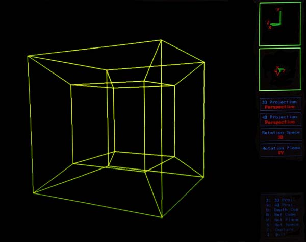
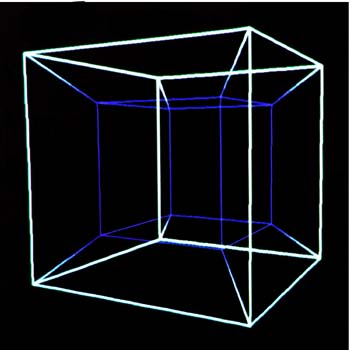
This analogy extends quite nicely to four-dimensional wireframes; the ``depth'' of a vertex is simply the 4D W eye-coordinate. As an example, when the four-cube is rendered with 4D depthcueing, the ``inner'' cube is shaded with a lower intensity than the ``outer'' cube, since it is farther away in four-dimensional space.
In figures 4.5a through 4.5d, the hypercube with vertices of <±1, ±1, ±1, ±1> is rendered with 4D parallel & perspective and 3D parallel & perspective projections. The four-cube is displayed with the following viewing parameters:
    From4  = <4, 0, 0, 0>
    To4    = <0, 0, 0, 0>
    Up4    = <0, 1, 0, 0>
    Over4  = <0, 0, 1, 0>
    theta4 = 45 degrees
    From3  = <3.00, 0.99, 1.82>
    To3    = <0, 0, 0>
    Up3    = <0, 1, 0>
    theta3 = 45 degrees
In figure 4.5a, the ``inner'' cube is actually farther away in four-space than the ``outer'' cube, and hence appears smaller in the resulting projection. You can think of the larger cube as the ``front face'' of the four-cube, and the the smaller cube as the ``rear face'' of the four-cube. When rotating the four-cube in the proper plane, the rear face gradually swings to the front, and the front face gradually swings to the rear. In doing this, the cube appears to turn itself inside out, so that the originally smaller cube engulfs the previously larger cube.
In figure 4.5c, the four-cube is displayed with 4D parallel projection and 3D perspective projection. Because of the parallel projection from 4D, the ``rear face'' and ``front face'' are displayed as the same size, so the parallel projection from this point in four-space looks like two identically-sized three-cubes superimposed over each other.
Figures 4.6a through 4.6d are similar to figures 4.5a through 4.5d, except that the four-dimensional viewpoint has changed. For these views, the four-dimensional viewing parameters are:
    From4  = <2.83, 2.83, .01, 0>
    To4    = <0, 0, 0, 0>
    Up4    = <-.71, .71, 0, 0>
    Over4  = <0, 0, 1, .02>
    theta4 = 45 degrees
    From3  = <3.29, .68, 1.4>
    To3    = <0, 0, 0>
    Up3    = <.08, 1, .04>
    theta3 = 45 degrees
This vantage point occurs one eighth of the way though a complete four-dimensional rotation. See figure 4.7a for an illustration of this rotation.
Figure 4.7a shows the sequence of one fourth of a four-dimensional rotation of the hypercube (read the sequence from top to bottom, left to right) with 4D and 3D perspective projection. Figure 4.7b shows the same sequence with 4D parallel and 3D perspective projection.
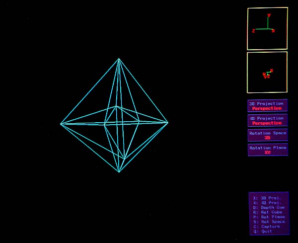
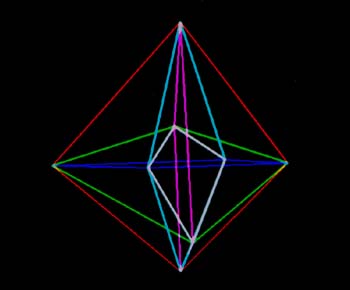
In figure 4.9, the dual of the four-cube is rendered with all edges rendered the same color. The dual of the four-cube is the wireframe of convex hull of the face centers of the four-cube. In other words, the convex hull of the points <±1, 0, 0, 0>, <0, ±1, 0, 0>, <0, 0, ±1, 0>, and <0, 0, 0, ±1>. One could also think of it as the four-dimensional analog of the three-dimensional octahedron.
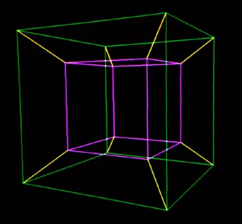
Figures 4.8 through 4.13 illustrate the differences in single edge-color rendering, multiple edge-color rendering, and depth-cued edge rendering. Even with interactive manipulation of the four-dimensional wireframe, single edge-color rendering yields an image that is difficult to interpret. Assigning different colors to the edges greatly aids the user in identifying sub-structures of the four-dimensional wireframe, and serves as a structural reference when rotating the object. Depth-cueing the edges gives a spatial sense of the object, but loses the structural cues.
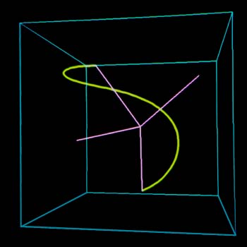
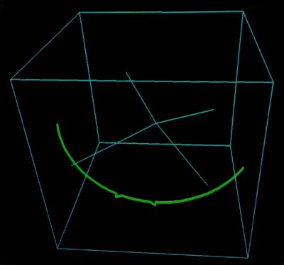
Finally, figures 4.14 and 4.15 show generalized curves across the surface of a four-sphere. The curve in figure 4.15 is given with poor uniform parameterization which yields the two ``kinks'' that are visible in the 4D image. For more information on these particular curves and the choices of parameterization, refer to [Chen 90].
| Previous Chapter | Table of Contents | Next Chapter |