The purpose of fire modeling is to gain a better insight into fire dynamics and how it impacts fire safety -- not to generate large amounts of data. Gaining this insight requires visualization tools that display what the numbers generated by the model represent. This article highlights some of the features that the visualization tool, Smokeview, uses to display fire effects.

Beginning in the early 1980s and continuing into the1990s, NIST researchers Howard Baum and Ron Rehm developed the basic flow solver that evolved into the Fire Dynamics Simulator, which was publicly released in 2000. Their solution technique, known as "large eddy simulation," or LES, captures very complicated fire plume dynamics. Early attempts to visualize the calculation results consisted of nothing more than little particles swirling about in a box. This was useful to the model developers but hardly to anyone else. It just did not look like a fire.

article continues below

Smokeview was written to address this problem. The first version was released along with FDS in early 2000. Along with particle-tracking as performed before, it visualized fire flow data by coloring and animating fire/smoke flow, making it much easier to interpret FDS simulation results. Immediately after September 11, 2001, work began on both FDS and Smokeview to enable them to model and visualize much larger problems. As a result, fire scenarios with several million grid cells can now be modeled and visualized using a cluster of computers.

The next big step in Smokeview's development was the implementation of an algorithm for visualizing smoke realistically. The line between FDS, which performs smoke flow computations, and Smokeview, which performs smoke flow visualization, became blurred as Smokeview now performs physics-based computations (Beer's law) in order to visualize the smoke. The present algorithm for visualizing smoke only considers the effects of absorption - how much an object is obscured by smoke. Future work involves modeling the effects of scattering - how the interaction between light nd smoke effects the visualization.

A 1999 townhouse fire that resulted in line-of-duty deaths for two firefighters can be used to illustrate how scientific visualization can be important.¹ NIST was asked by the District of Columbia Fire and Emergency Medical Services Department Reconstruction Committee to examine the fire dynamics of this incident. The Committee had several questions regarding: 1) the injuries that the firefighters had sustained; 2) the lack of thermal damage in the living room where the fallen firefighters were found; and, 3) why the firefighters never opened their hose-lines to protect themselves and extinguish the fire. The major source of confusion arose from the fact that the firefighter farthest from the fire died while the one in the middle (closer to the fire) survived. 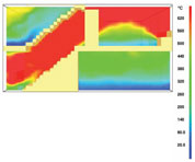Figure 1 shows that one-dimensional thinking is not always valid. This figure shows temperature contours through the center line of a basement stairwell. The heated gases moved up the basement stairs due to buoyancy and arched over the firefighters located at the top of the stairs. This visualization makes it clear that the fire dynamics was not one-dimensional and that conditions for the middle firefighter were less hazardous than conditions for the other two.

SIMULATION OVERVIEW
NIST, the National Institute of Standards and Technology, has developed a suite of validated computational tools for the simulation and visualization of fire spread and smoke transport. One of the fire modeling tools is called the Fire Dynamics Simulator (FDS).^2,3 Developed as a companion to FDS, Smokeview is a scientific visualization tool that converts data to images, enabling one to better understand numerically predicted fire dynamics.^4,5 These tools were developed with an emphasis on ease of use on affordable computer platforms.

FDS predicts smoke and/or hot air flow movement caused by fire, wind, ventilation systems and other factors by numerically solving the fundamental equations governing fluid flow, commonly known as the Navier-Stokes equations. FDS uses a form of computational fluid dynamics (CFD) known as large eddy simulation (LES) to predict the thermal conditions resulting from a fire. LES is a way of describing the effect of turbulence on the flow field. The fire itself is a source term in the governing equations, creating buoyant motion that drives the smoke and hot gases throughout the simulation. The chemistry of the combustion process is complicated by the fact that the fuel for the fire may include room furnishings, ceiling materials, wall and floor coverings, etc., i.e., a wide assortment of different materials. FDS makes simplifications about the combustion, essentially saying that fuel and oxygen burn readily when mixed. The rate at which energy is generated is obtained from experiments. There is no attempt to model the fundamental chemistry, which can involve hundreds of chemical reactions.

Both FDS and Smokeview would not have been possible without the recent advent of high-speed computers for performing computations, fast video cards for visualizing results and the Internet for exchanging information and ideas. These programs also would not have been possible without the research needed to develop the underlying fire models and the techniques needed to implement these models accurately and efficiently.

VISUALIZATION OVERVIEW
One of the biggest challenges in visualizing fire dynamics is how to convert the multidimensional data generated by a fire model such as FDS into a form that can be easily understood. Fire data can easily have five or more dimensions. For example, to display time-dependent scalar data would require five dimensions: three spatial dimensions to visualize position, one time dimension and one dimension to visualize the variable of interest. Time-dependent vector quantities require eight dimensions to display: three spatial dimensions, one time dimension, one dimension to visualize the variable, plus three additional dimensions to display the flow direction and speed.

A major challenge to effective visualization is that the computer screen has only two dimensions to display these data. A third dimension may be conveyed by rapidly displaying a sequence of images, with each image representing a different moment in time. The visualization challenge is even more difficult when conveying results for the printed page.

Smokeview visualizes data in two primary ways: quantitative and realistic. Quantitative methods typically map fire modeling data into colors representing a fire modeling variable. Interpreted with a color bar, one can make quantitative assessments about the data being examined. Some examples used by Smokeview are animated tracer particles; animated two-dimensional slices of gas phase quantities, such as temperature or smoke concentration; animated flow vectors; and animated surface conditions, such as incident heat flux or burning rates on enclosure surfaces. 3-D level or isosurfaces are also used to indicate where a particular variable takes on a specified value. Smokeview also visualizes smoke realistically by converting soot density to smoke opacity, with the goal of displaying smoke as it would actually appear to an observer. Each of these visualization techniques highlights different aspects of the underlying flow phenomena.

Visualization is essential at all stages of the modeling process. It is used before a run to verify the correctness of the scenario geometry, (e.g., locations and size of simulation features), during a run to monitor the simulation (ensuring boundary flows are behaving as intended) and after the run has been completed to analyze the results.

QUANTITATIVE VISUALIZATION

Showing motion
FDS uses particles to simulate water droplets and fuel sprays. One may also introduce particles into a scenario as tracers. All three particle types may be visualized using Smokeview, revealing the underlying flow patterns of the simulation.

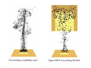
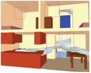
Fluid motion may be conveyed by displaying a sequence of still images. A single static particle image, however, is not a good method for showing motion. The two cases shown in Figure 2 both display particles generated by a fire plume. The surroundings in the top illustration are completely open, while the upper half of the domain in the lower illustration is enclosed. The particle pattern in both cases looks similar though the fire dynamics are quite different.

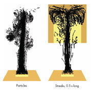
Streak lines, a new feature of Smokeview version 5, are a good method for showing motion in a static image. A streak line is simply the path a particle takes due to the changing underlying flow field. (If the flow field was unchanging, then these lines would be called stream lines.) The streak lines shown in Figure 3 indicate how particles are affected by the boundary conditions. Streaks are predominantly vertical in the left illustration, since the domain boundary is completely open, while the streaks are curved near the top of the illustration on the right since the upper half of the domain boundary is blocked.

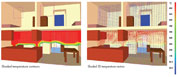
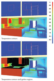
A second method for showing motion is the use of animated flow vectors. The vector's color represents the data, and the vector's length and direction show the dynamics of the underlying flow field. Figure 4 shows the fire dynamics of a kitchen fire using both solid shaded contours and a vector plot. Vector plots are better than solid contours for highlighting flow changes, especially in regions where temperatures are uniform.

Assessing variables
Within the Gas Phase. Smoke-view allows animated shaded color contours of calculated gas quantities to be drawn at any horizontal or vertical plane in the simulation. To minimize file output, the user specifies the particular slice planes to be visualized. If disk space is not an issue, then the user may specify the entire 3D volume. Smokeview then allows the user to scroll through the 3D volume of data one slice at a time, displaying any horizontal or vertical plane. The lower illustration in Figure 4 illustrates temperature contours in a vertical plane through the center of a static townhouse kitchen fire (not the Cherry Road case). Regions where the temperatures are below 100°C are hidden. Hiding unimportant data is a good technique for eliminating the data that is important.

On Surfaces. Boundary files contain simulation data recorded at blockage or wall surfaces. Continuously shaded contours are drawn for quantities such as wall surface temperature, radiative flux, etc. Figure 5 shows a snapshot of a boundary file animation where the surfaces are colored according to their temperature.

Regions where a surface temperature exceeds its ignition temperature (where burning has occurred) may be colored black. This is also illustrated in Figure 5.

Particular Locations. Smokeview uses isosurfaces to identify where a specified level of a gas phase quantity occurs rather than how much. For example, FDS uses a mixture fraction model to simulate combustion. In this model, there is a critical or stoichimetric mixture fraction value, such that regions greater than the critical value are fuel-rich and regions less than the critical value are fuel-lean. Burning then occurs, according to the model, on the level surface where the mixture fraction equals this stoichimetric value. Therefore, it is of interest to visualize these locations.

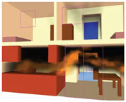
Another application of isosurfaces is to identify where in the simulation domain a particular temperature occurs. This temperature could represent a hazard or a condition when something happens such as a smoke or heat detector activating. Figure 6 shows the region in a town-house kitchen fire where the temperature is 100°C. The time and view point are the same as shown Figure 4.

Realistic visualization
Visualizing smoke realistically is challenging for three reasons. First, the storage requirements for describing smoke throughout the simulation scene at every time step can easily exceed the file size capacities of present 32-bit operating systems, which would typically be 2 GB. Second, the computation required both by the CPU and the video card to display each frame can easily exceed 0.1 s, the time corresponding to a 10 frame/s display rate. Finally, the physics required to describe smoke and its interaction with itself and surrounding light sources is complex and computationally intensive. Approximations and simplifications are required.

Smoke visualization techniques described previously, such as the use of tracer particles or shaded 2-D contours, are useful for analyzing data quantitatively but are not suitable for applications where realism is required. Some examples of such applications are using Smokeview as a virtual firefighter trainer or using Smokeview to examine the obscuration effects of smoke. Figure 7 shows smoke and fire displayed realistically.

References:

1. Madrzykowski, D., and Vettori, R., "Simulation of the Dynamics of the Fire at 3146 Cherry Road NE, Washington, DC, May 30, 1999." NISTIR 6510, National Institute of Standards and Technology, Gaithersburg, MD, 2000.
2. McGrattan, K., et al., "Fire Dynamics Simulator (Version 5), User's Guide." NIST Special Publication 1019-5, National Institute of Standards and Technology, Gaithersburg, MD, 2007.
3. McGrattan, K., et al., "Fire Dynamics Simulator (Version 5), Technical Reference Guide." NIST Special Publication 1018-5, National Institute of Standards and Technology, Gaithersburg, MD, 2007.
4. Forney, D., et al., "Understanding Fire and Smoke Flow Through Modeling and Visualization." Computer Graphics and Applications, 23(4):6--13, 2003.
5. Forney, G., et al., "User's Guide for Smokeview Version 5 - A Tool for Visualizing Fire Dynamics Simulation Data." NIST Special Publication 1017-5, National Institute of Standards and Technology, Gaithersburg, MD, June 2007.